Purpose and Need
" Historically, ideas from linear programming have inspired many of the central concepts of optimization theory, such as duality, decomposition, and the importance of convexity and its generalizations."
Many practical problems in operations research can be expressed as linear programming problems. There is a large need for linear programming in microeconomics and company management, such as planning, production, transportation, technology and other issues. While most modern management issues are constantly changing, most companies would still like to maximize profits or minimize costs with limited resources. Therefore, many companies can utilize linear programming by characterizing their issues in this way.
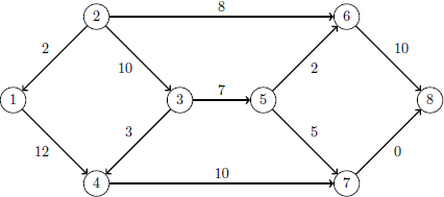
Because a large variety of problems in Operations Research can be expressed as linear programming problems, linear programming is mostly use in the filed of optimization. The most common type of problems in Operations Research that are expressed as linear programming problems are network flow problems and the diet problem. A network flow problem is about finding the maximum output in a flow. This can be used to find the optimal flow of cars in a road system, fluids in pipelines, and anything that travels through a network with limitations on flow. A diet problem is a model where the goal is to find the optimal value while having multiple constraints. For example, on a menu with food, all the items on the menu have different vitamins, minerals and other nutrients. The optimal output being the lowest cost while completing all the goals of having sufficient nutrients in the food menu items. As you can see there are many purposes and needs for linear programming.
Many practical problems in operations research can be expressed as linear programming problems. There is a large need for linear programming in microeconomics and company management, such as planning, production, transportation, technology and other issues. While most modern management issues are constantly changing, most companies would still like to maximize profits or minimize costs with limited resources. Therefore, many companies can utilize linear programming by characterizing their issues in this way.
Because a large variety of problems in Operations Research can be expressed as linear programming problems, linear programming is mostly use in the filed of optimization. The most common type of problems in Operations Research that are expressed as linear programming problems are network flow problems and the diet problem. A network flow problem is about finding the maximum output in a flow. This can be used to find the optimal flow of cars in a road system, fluids in pipelines, and anything that travels through a network with limitations on flow. A diet problem is a model where the goal is to find the optimal value while having multiple constraints. For example, on a menu with food, all the items on the menu have different vitamins, minerals and other nutrients. The optimal output being the lowest cost while completing all the goals of having sufficient nutrients in the food menu items. As you can see there are many purposes and needs for linear programming.
HOW IT WORKS
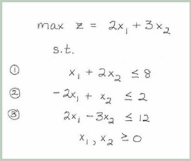
We will begin with a simple example of how linear programming works with a simple problem with two decision variables. The procedure is usually similar to this:
Step 1: Graph the constraints
Step 2: Identify the feasible region
Step 3: Determine the slope of the objective function
Step 4: Identify the optimal point
Step 5: Find the coordinates of the optimal point
Step 6: Substitute the coordinates into the objective function to find the value of the objective function at the optimal solution.
This will be the example problem we will be using for the remainder of the steps.
Step 1: Graph the Constraints
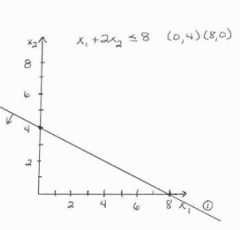
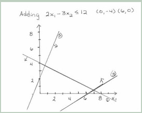
For each constraint, you first graph the line that corresponds to the constraint as an equality. Second, you determine which side of the line is the feasible area that satisfy the inequality. You can graph the line that corresponds to the constraint written as an equality or by replacing one variable with a zero and getting the opposite variable value, then doing the same to the other variable. For example, to get the x,y coordinate for the first constraint, I would first set x1 to zero and the resulting x2 would be 4. Then I would set x2 to zero and the resulting x1 would be 8. This is represented by graph one.. Traditionally we label the horizontal axis as x1 and the vertical axis as x2.
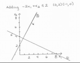
To determine which side of the line contains points that satisfy the inequality, pick a point that is on one side of the line and substitute those values into the constraint. If the constraint is met, then that is the side that is shaded, if the constraint is not met, then that is not the feasible region. Do not make the mistake of assuming that the area below or to the left of the line will be shaded for less than or equal constraints; this is not always the case.
Next we add the second and third constraint using the same graphical approach. The resulting graphs are shown in graph two for constraint two, and graph three for constraint three.
|
Graph One
|
Graph Two
|
Graph Three
|
Step Two: Identify the Feasible Region
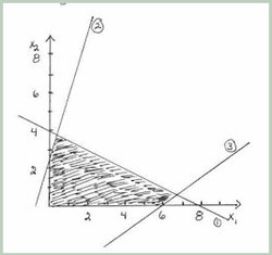
Graph Four
Now we want to shade in the feasible area. This is the area that meets all the constraints. You will find this by determining the side of each constraint that satisfies the inequality. In this case it will be below the first constraint line, to the left of the second constraint line, and to the right of the third constraint line. This region is shown in graph four to the left.
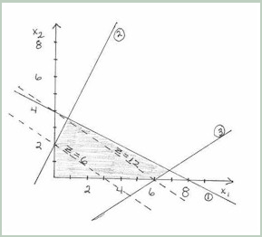
Step Three: Determine the Slope of the Objective Function
To determine the slope of the objective function, it is simply the negative coefficient of x1 over the coefficient of x2. In our case this is -2/3. From this slope, we will be able to find the optimal point on our graph. Graph the optimal solution line, take a ruler, and continue moving outward. As you can see from graph five, the further and further we take the objective function line out, the last point it reaches will be our optimal solution.
|
Graph Five
|
Step Four, Five, and Six
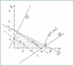
As I said above, the last point that the optimal line touches will be the optimal point. In this case, as you can see from graph six, the optimal solution lies at the intersection of constraint one and constraint three. You can solve this equation by setting them equal to each other or subtracting them from each other. Once you have determined the x and y values, plug those into the objective function and you will get your optimal solution.
